PCA details
In machine learning, threre are many features can be used for training. For example, we have 72 features in each instance and 1000 pieces of data. So now we have a matrix D with shape of (1000, 72). If we want to reduce the feature number, then we need another matrix R and compute dot product: $D * R = D^{‘}$ Suppose the shape of R is (72, 30), and the $D^{‘}$ is in (1000, 30). So the now our task is to find a good $R$ to keep as much information as possible.
Maximum variance
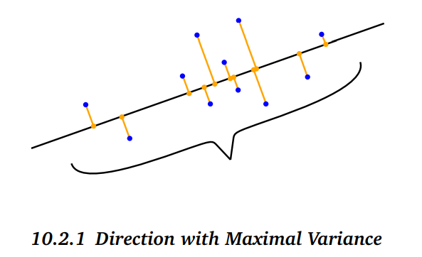
Pic from Marc Peter Deisenroth, A. Aldo Faisal, Cheng Soon Ong, 2020
We can see if wee want to reduce dimension form 2 to 1, the best line is what is shown in the picture. This is understandable because the projections of dots are more discrete. Let’s consider an opposite case, say the line is perpendicular to the original one. Then the projects lie on a very narrow area, for example, they are [1, 0] [1.5, 0], [1, 0] [-1, 0] [1, 0] [-0.5, 0], which are ineffective to represent original points because a lot of them look exactly the same.
Therefore, we wish the projection has the max variance so that most information is kept.
Covariance
Based on above discussion, we should be able to know the task is to find a plane where the variance is max. Variance formula is as follows
\[\begin{equation} S = \frac{1}{N-1} \Sigma_{i}^{N} (x_{i}-\bar{x})^{2} \end{equation}\]Where N is the number of dimensions.
If we change the equation a little bit, then it turns to $Cov(x,y)=\frac{1}{N-1} \Sigma_{i}^{N} (x_{i}-\bar{x})*(y_{i}-\bar{x})$ which is a covairance matrix. When x = y the value is actually the variance of x.
Before we do the projection, we must first standardize the data, then do the projection and maximize the variance.
\[\begin{equation} \begin{aligned} J &= \frac{1}{N-1}\Sigma_{i=1}^{N} ((x_{i}-\bar{x})\mu)^{2}\\ &= \frac{1}{N-1}\Sigma_{i=1}^{N} \mu^{T}(x_{i}-\bar{x})^{T}(x_{i}-\bar{x})\mu \\ &= \mu^{T} \frac{1}{N-1}\Sigma_{i=1}^{N} (x_{i}-\bar{x})^{T}(x_{i}-\bar{x})\mu \\ &= \mu^{T}S\mu \end{aligned} \end{equation}\]Where $\mu$ is the $R$ we mentioned in previous section. There is another property for $\mu$: $\mu^{T}\mu = 1$ which results from the fact that covariance matrix is always a systematric square.
Then the whole question becomes an optimization problem. To find the best $\mu$ so that the $J$ is maximum variance.
\[argmax (J) = \mu^{T}S\mu\] \[s.t. \: \mu^{T}\mu = 1\]Use Lagrange multiplier to solve the problem.
\[L(\mu, \lambda) = \mu^{T}S\mu +\lambda(1-\mu^{T}\mu) \\\]The equation is max when the following requirement(just one of them, but enough) is met.
\[\frac{\partial L}{\partial \mu} = 2S\mu - 2\lambda \mu =0\]The result is $S\mu = \lambda \mu$ which indicates $\lambda$ stands for eigenvalues of $S$, and $\mu$ for eigenvectors.
By computing eigenvectors corresponding to top X largest eigenvalues, we obtain the $\mu$ to reduce dimensions.
Eigenvalue & Eigenvector
Definition: $A x = \lambda x$ => $|A - \lambda E|=0$
The $\lambda$ holds the equation is eigenvalue and the $x$ is eigenvector.
- $A$ should be a square matrix.
- If $A(n,n)$ is not invertible ($A$ is singular, rank is less than n), there must be at least one $\lambda$ is zero.
For example, now square matrix
\[A=\left[ \begin{matrix} 12 & 8 \\ 5 & 6 \\ \end{matrix} \right]\] \[\begin{aligned} |A - \lambda I| &= det \left\{ \left[ \begin{matrix} 12-\lambda & 8 \\ 5 & 6-\lambda \\ \end{matrix} \right] \right\} \\ &=(12-\lambda)(6-\lambda)-5*8 \\ &= \lambda^{2} - 18\lambda + 72 - 40 \\ &= \lambda^{2} - 18\lambda + 32 \\ &= (\lambda -16)(\lambda -2)\\ \end{aligned} \\\]So the $\lambda_{1}=2, \lambda_{2}=16$ and the $x_{1}=\begin{bmatrix} -4 \ 5 \end{bmatrix}$ and $x_{2}=\begin{bmatrix} 2 \ 1 \end{bmatrix}$
But here is a restriction that the matrix has to be a N x N matrix. However, in reality there are many matrices in shape of N x M.
SVD
Singular value and vector
Consequently, singular values and vectors are designed for those matrices whose rows(N) are different from columns(M).
Suppose we can decompose $A=U\Sigma V^{T}$, where $U$ and $V$ are both orthogonal. Then the followings also hold
- $AA^{T}=U\Sigma V^{T}(U\Sigma V^{T})^{T}=U\Sigma V^{T}V\Sigma U^{T}=U\Sigma \Sigma U^{T}$
- $A^{T}A=(U\Sigma V^{T})^{T}U\Sigma V^{T}=V\Sigma U^{T}U\Sigma V^{T}=V\Sigma \Sigma V^{T}$
So the singular values are the root square of $\Sigma$ values. For example,
\(A=\left[ \begin{smallmatrix} 3 & 2 \\ 2 & 3 \\ 2 & -2 \\ \end{smallmatrix} \right]\)
and \(A^{T}=\left[ \begin{smallmatrix} 3 & 2 & 2 \\ 2 & 3 & -2 \\ \end{smallmatrix} \right]\)
We first calculate the $V$
\[\begin{aligned} A^{T}A &=\left[ \begin{matrix} 3 & 2 & 2 \\ 2 & 3 & -2 \\ \end {matrix}\right]*\left[ \begin{matrix} 3 & 2 \\2 & 3 \\ 2 & -2 \\\end{matrix}\right] \\ &= \left[ \begin{matrix} 17 & 8 \\ 8 & 17 \\\end {matrix}\right] \end{aligned}\]$det(A^{T}A)=\lambda^{2}-34\lambda+289-64=(\lambda -9)(\lambda-25)$ so the singular value $q_{1}=\sqrt 9 = 3$ and $q_{2}=\sqrt 25 = 5$ and we rank the singular values:
\(v_{1}=\frac{1}{\sqrt 2} \begin{bmatrix} 1 \\ -1 \\ \end{bmatrix}, v_{2}=\frac{1}{\sqrt 2} \begin{bmatrix} 1 \\ 1 \\ \end{bmatrix} , V=\begin{bmatrix} 1 & 1 \\ 1 & -1 \\ \end{bmatrix}, \Sigma= \begin{bmatrix} 5 & 0 \\ 0 & 3 \\ \end{bmatrix}\)
According to $U=AV\Sigma^{-1},\; u_{i}=\frac{Av_{i}}{\sigma_{i}}$, we know:
\[\begin{aligned} u_{1}&=\frac{\left[ \begin{matrix} 3 & 2 \\2 & 3 \\ 2 & -2 \\\end{matrix}\right]*\frac{1}{\sqrt 2}\left[ \begin{matrix} 1 \\ 1 \\\end {matrix}\right]}{5} &=\frac{1}{\sqrt 2}\left[ \begin{matrix} 1 \\ 1 \\ 0 \end {matrix}\right] \\ u_{2}&=\frac{\left[ \begin{matrix} 3 & 2 \\2 & 3 \\ 2 & -2 \\\end{matrix}\right]*\frac{1}{\sqrt 2}\left[ \begin{matrix} 1 \\ -1 \\\end {matrix}\right]}{3} &= \frac{1}{\sqrt 2} \left[ \begin{matrix} 1/3 \\ -1/3 \\ 4/3 \end {matrix}\right] \end{aligned}\]And the
\[U=\frac{1}{\sqrt 2}\begin{bmatrix} 1 & 1/3 \\ 1 & -1/3 \\ 0 & 4/3 \\ \end{bmatrix}\]And now we can verify:
\[U\Sigma V^{T}=\frac{1}{\sqrt 2}\begin{bmatrix} 1 & 1/3 \\ 1 & -1/3 \\ 0 & 4/3 \\ \end {bmatrix}* \begin{bmatrix} 5 & 0 \\ 0 & 3 \\ \end{bmatrix} * \frac{1}{\sqrt 2} \begin{bmatrix} 1 & 1 \\ 1 & -1 \\ \end{bmatrix} =\frac{1}{2} \begin{bmatrix} 6 & 4 \\ 4 & 6 \\ 4 & -4 \\ \end{bmatrix}=A\]Application
So in which way can it be used? The general form of SVD is:
\(\begin{bmatrix} a_{11} & a_{12} & \cdots & a_{1m} \\ a_{21} & a_{22} & \cdots & a_{2m} \\ \vdots & \vdots & \ddots & \vdots \\ a_{n1} & a_{n2} & \cdots & a_{nm}\\\end {bmatrix}_{(n \times m)} = \left[ \begin{matrix} u_{11} & \cdots & u_{1k} \\ \vdots & \ddots & \vdots\\ u_{n1} & \cdots & u_{nk}\\\end {matrix}\right]_{(n \times k)} \left[ \begin{matrix} \sigma_{1} & 0 & \cdots & 0 & 0 \\ 0 & \sigma_{2} & \cdots & 0 & 0\\ \vdots & \vdots & \ddots & \vdots & \vdots \\ 0 & 0 & \cdots & \sigma_{k-1} & 0 \\ 0 & 0 & \cdots & 0 & \sigma_{k}\\\end {matrix}\right]_{(k \times k)} \left[ \begin{matrix} v_{11} & \cdots & v_{1k} \\ \vdots & \ddots & \vdots\\ v_{m1} & \cdots & v_{mk}\\\end {matrix}\right]^{T}_{(k \times m)}\) where $\sigma_{i}$ is ranked by value from high to low, which indicates the contribution of $\sigma_{i}$.
Sometimes the last several values like $\sigma_{k}$ are quite small/close to 0, and they can be just removed. And the form is:
This way of decomposition saves the most information of matrix.
Python code
By running the following code, it shows the original picture
1
2
3
4
5
6
7
from PIL import Image
import numpy as np
import matplotlib.pyplot as plt
tower=Image.open("SVD-origin.jpg","r")# file name could be replaced
tower_pixel_matrix=np.asarray(tower)
plt.figure(figsize=(9, 9))
plt.imshow(tower)

1
2
3
4
5
6
7
8
x,y,z=tower_pixel_matrix.shape
tower_pixel_matrix = tower_pixel_matrix.reshape(x,y*z)
U, sigma, V=np.linalg.svd(tower_pixel_matrix)
fig,ax=plt.subplots(nrows=2, ncols=2,figsize=(12,8))
for k in [(0,0,10),(0,1,20),(1,0,100),(1,1,500)]:
    blurred_tower = np.matrix(U[:, :k[2]]) * np.diag(sigma[:k[2]]) * np.matrix(V[:k[2], :])
    ax[k[0],k[1]].imshow(blurred_tower)
    ax[k[0],k[1]].title.set_text("Key components:{}".format(k[2]))
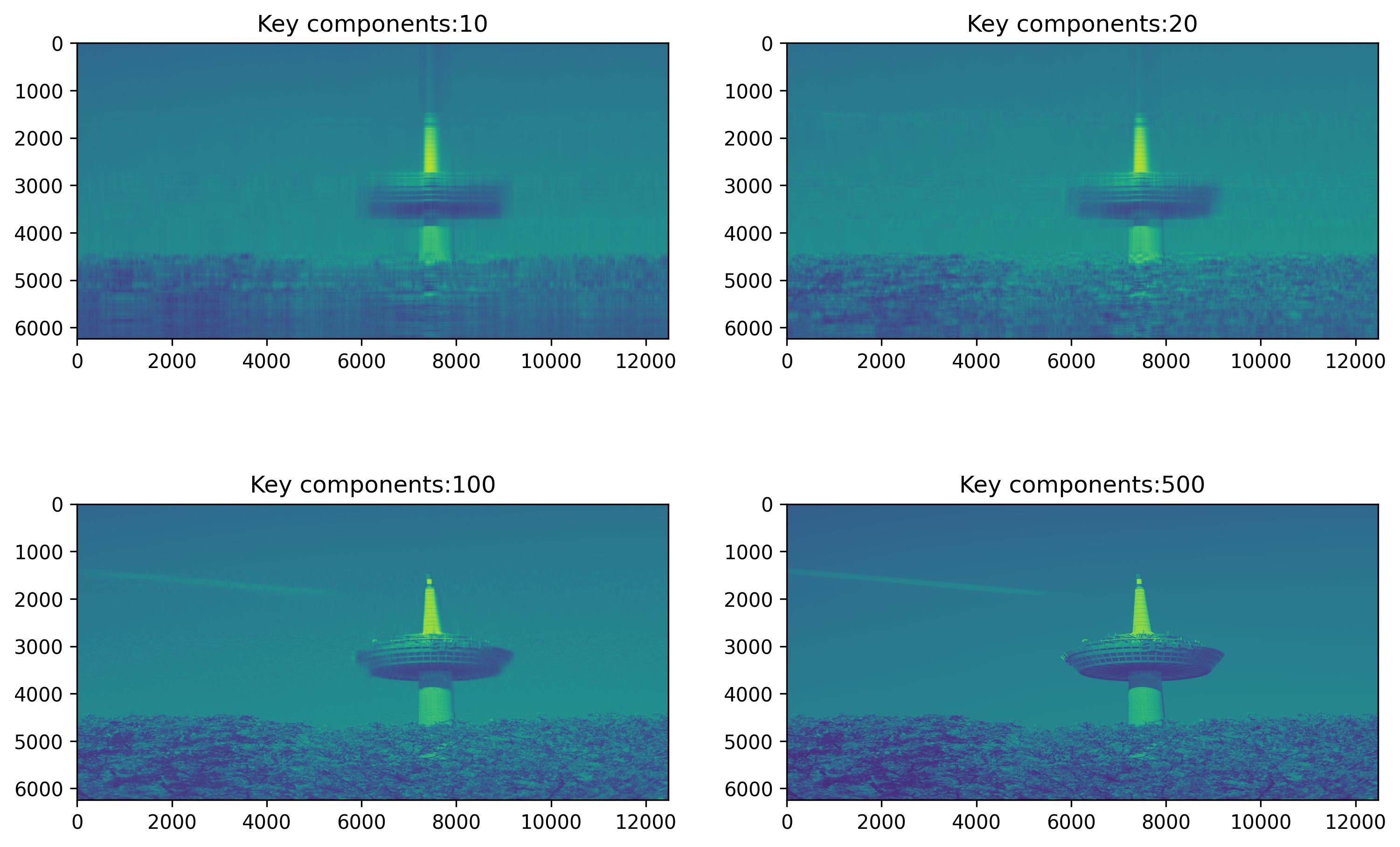
It’s clear that key components save the most important information, like the outline of objects. The more components are saved, the more details are provided.
sklearn provides API for SVD as well. This approach is usually applied to reduce dimensions of data at the least cost. It’s a very useful method in machine learning. This method can also be used in NLP field. For example, Latent Semantic Analysis(LSA) uses SVD to map the term-document on certain space and grouping words of similar semantic meaning.